pacman::p_load(ggstatsplot, plotly, tidyverse)Take Home Exercise 3
1. Overview
The purpose of the exercise is to uncover the salient patterns of resale prices of public housing property by residential towns and estates in Singapore. I will use select appropriate analytical visualisation techniques to discover the similarity and difference of data pattern for 3-Room, 4-Room and 5-Room flats. The study period is base on 2022 resale data that is available on data.gov.sg named “resale-flat-prices-based-on-registration-date-from-jan-2017-onwards”.
2. Visualization Tool Selection
In this exercise, I will apply different univariate graphical method and bivariate method and appropriate statistical testing to discover housing price pattern of different flat type and geographic location.
Univariate Graphic EDA
1) Histogram on housing prices distribution:
This is to discover if the housing prices and transactions are normally distributed. I will build a static chart to reveal the distribution, and interactive charts to unveal more information, and statistical test on normal distribution.
Multivariate Graphic EDA
2) Boxplot
This is to discover the different means and percentile of housing prices for different independent categorical variable such as room type, flat model and geographic location. I will use boxplot and statistical method such as Oneway ANOVA to prove the hypothesis if different group shares the same mean and pattern.
a) Compare resale flat prices for 3-Room, 4-Room and 5-Room flat
b) Compare resale flat prices between different town
c) Compare resale flat prices between different flat model
3) Correlation Analysis
This is to discover the relationship of housing prices and independent continuous variable such as house size and lease years. I will use scatterplot and calculate the correlation between the two variables.
a) Floor sq vs resale flat price per sqm
b) Remaining lease years vs resale flat price per sqm
Other Analysis
I will use Mosaic plot to show the relationship of different categorical variables (such as X & Y) to discover more insights on the housing patterns.
3. Step by Step Procedures
3.1 Getting Ready
In this exercise, ggstatplot, plotly and tidyverse will be used.
3.2 Import data
resale-flat-prices-jan2017.csv data is imported using tidyverse package
flat_data <- read_csv("data/resale-flat-prices-jan2017.csv")3.3 Data Transformation
In this exercise, we will only focus on 3-room, 4-room and 5-room flat as they share similar characteristic, the study period is 2022. Below code chunk help us to filter the selected data.
filter_data <- flat_data %>%
  filter(flat_type %in% c("3 ROOM", "4 ROOM", "5 ROOM")) %>%
  filter(str_detect(month,"2022"))
I also need to transform the resale price to resale price per sqm for fair comparison In the below code chunk, I created a new attributes called resale_price_per_sqm.
new_flat_data <- filter_data %>%
  mutate(resale_price_per_sqm = resale_price/floor_area_sqm)
In the code chunk below, I transform the char string in remaining_lease to numbers, capturing the remaining lease years for the later correlation analysis.
new_flat_data <- new_flat_data|>
  mutate(remaining_lease_years = parse_number(remaining_lease))
3.3 Histogram
3.3.1 Static Histogram
In the code chunk below, ggplot2 is used to build a histogram for “Distribution of Resale Flat Price” with mean resale flat price per sqm plotted as the X intercept.
m = mean(new_flat_data$resale_price_per_sqm)

ggplot(data=new_flat_data,
             aes(x = resale_price_per_sqm)) +
  geom_histogram(bins=50,
                 boundary = 100,
                 color="grey25",
                 fill="grey90") +
  geom_vline(aes(xintercept = mean(resale_price_per_sqm))) +
  ggtitle("Distribution of Resale Flat Price Per SQM")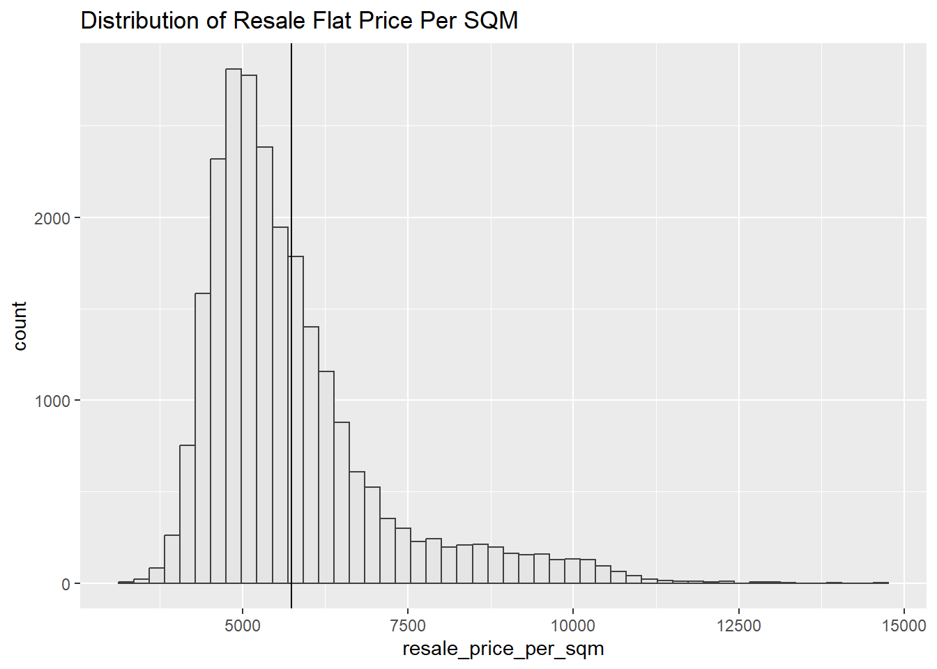
3.3.2 Interactive
In the code chunk below, ggplot2 is used to build a histogram for “Distribution of Resale Flat Price” using plotly. We color the bars with different room type to discover if there are different patterns.
plot_ly(data = new_flat_data,
        x = ~resale_price_per_sqm,
        color = ~flat_type)
3.3.3 One-sample test for normal distribution
In the code chunk below, gghistostats() is used to build a visual of one-sample test on housing prices.
set.seed(1234)

gghistostats(
  data = new_flat_data,
  x = resale_price_per_sqm,
  type = "bayes",
  test.value = 100,
  xlab = "HDB flat resale price"
)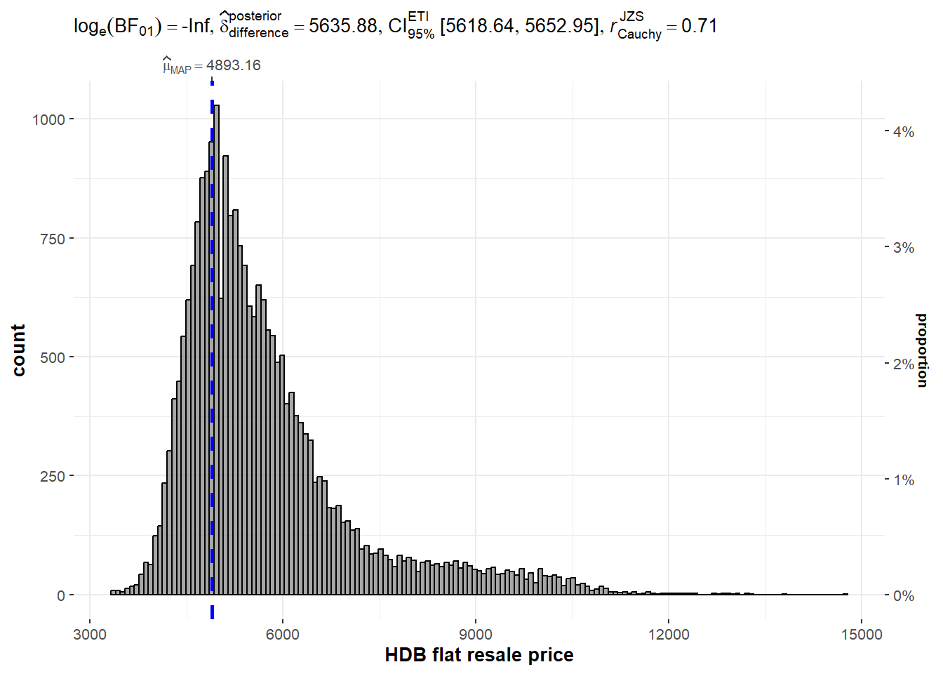
It shows an abecadotal evidence for alternative hypothesis according to Bayes Factor, which suggest the resale flat price is not normally distributed.
3.4 Boxplot
3.4.1 Mean resale flat price for different room type
In the code chunk below, geom_boxplot() is used to display the distribution of different room types (3-Room, 4-Room and 5-Room). For easier reading, the Y axis value are format in $K unit
ggplot(new_flat_data, aes(x = flat_type, y = resale_price_per_sqm)) +
  geom_boxplot() +
  scale_y_continuous(
    labels = scales::label_dollar(scale = 1/1000, suffix = "K"),
    breaks = seq(2000, 20000, by = 2000)) +
  ggtitle("Mean Comparison for Different Flat Type")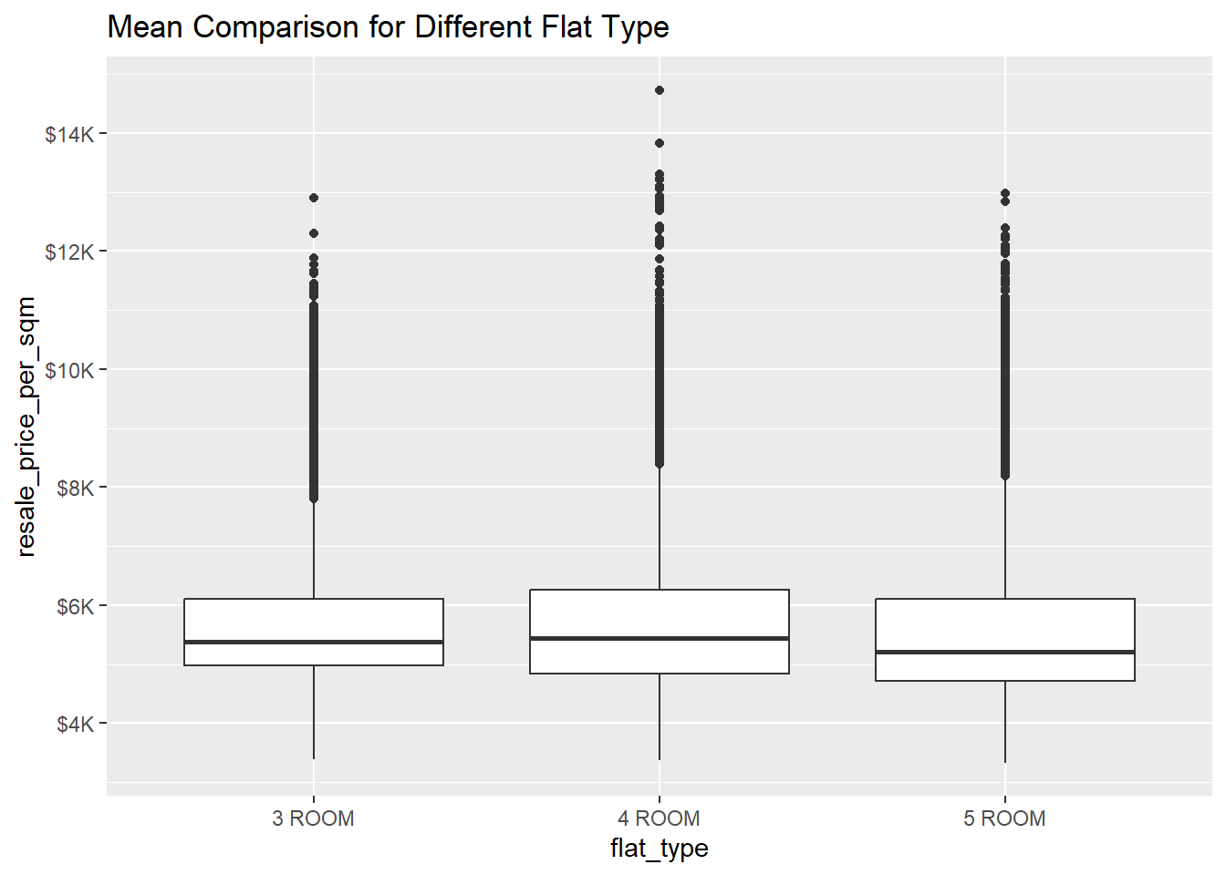
As the means and the data pattern for the 3 types of room looks the same, below code chunk is used to create a visual statistic testing to prove if different flat types share the same mean with Oneway ANOVA test using ggbetweenstats() method.
ggbetweenstats(
  data = new_flat_data,
  x = flat_type,
  y = resale_price_per_sqm,
  type = "p",
  mean.ci = TRUE,
  pairwise.comparisons = TRUE,
  pairwise.display = "s",
  p.adjust.method = "fdr",
  messages = FALSE
)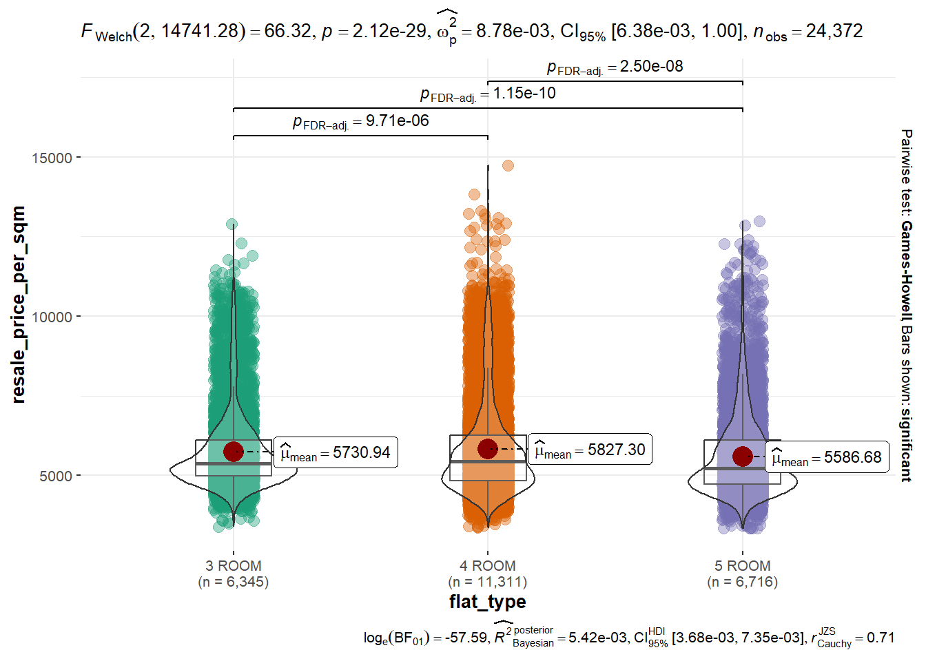
From the analysis above, we an see the result is significant which statistically prove that different flat types share the same mean resale price per sqm.
3.4.2 Mean resale flat price for different town
In the code chunk below, boxplot of flat price for different town are displayed for comparison. For easier reading, the Y axis value are format in $K unit and X axis title are rotated 90 degree.
ggplot(new_flat_data, aes(x = town, y = resale_price_per_sqm)) +
  geom_boxplot() +
  scale_y_continuous(
    labels = scales::label_dollar(scale = 1/1000, suffix = "K"),
    breaks = seq(2000, 20000, by = 2000)) +
  ggtitle("Mean Comparison of Resale Flat Price per sqm for Different Town") +
  theme(axis.text.x = element_text(angle = 90, vjust = 1, hjust=1), plot.title = element_text(hjust = 0.5))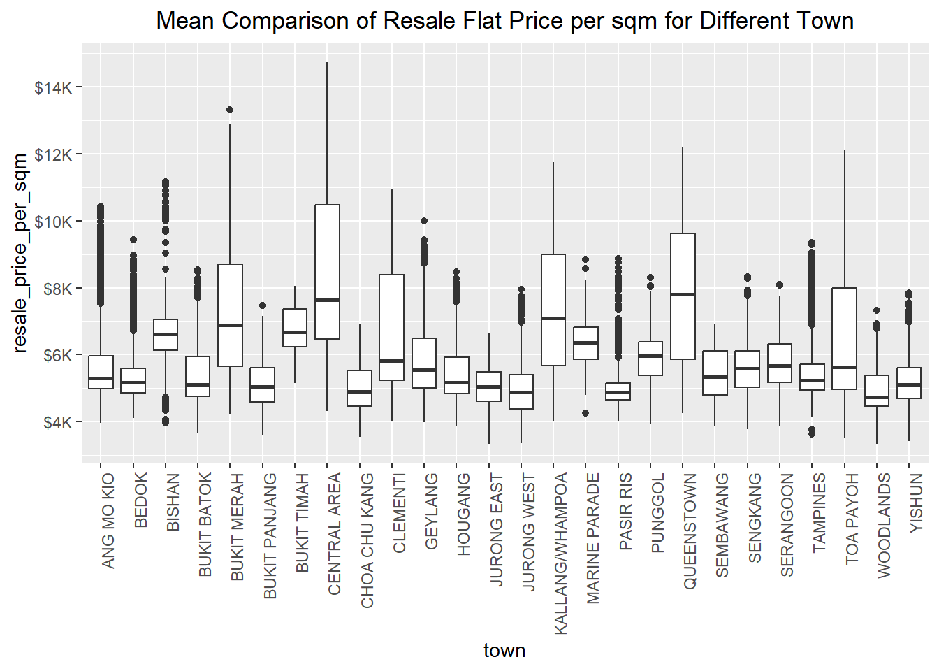
3.4.3 Mean resale flat price for different flat type
In the code chunk below, boxplot of flat price for flat models are displayed for comparison. For easier reading, the Y axis value are format in $K unit and X axis title are rotated 90 degree.
ggplot(new_flat_data, aes(x = flat_model, y = resale_price_per_sqm)) +
  geom_boxplot() +
  scale_y_continuous(
    labels = scales::label_dollar(scale = 1/1000, suffix = "K"),
    breaks = seq(2000, 20000, by = 2000)) +
  ggtitle("Mean Comparison of Resale Flat Price per sqm for Flat model") +
  theme(axis.text.x = element_text(angle = 90, vjust = 1, hjust=1), plot.title = element_text(hjust = 0.5))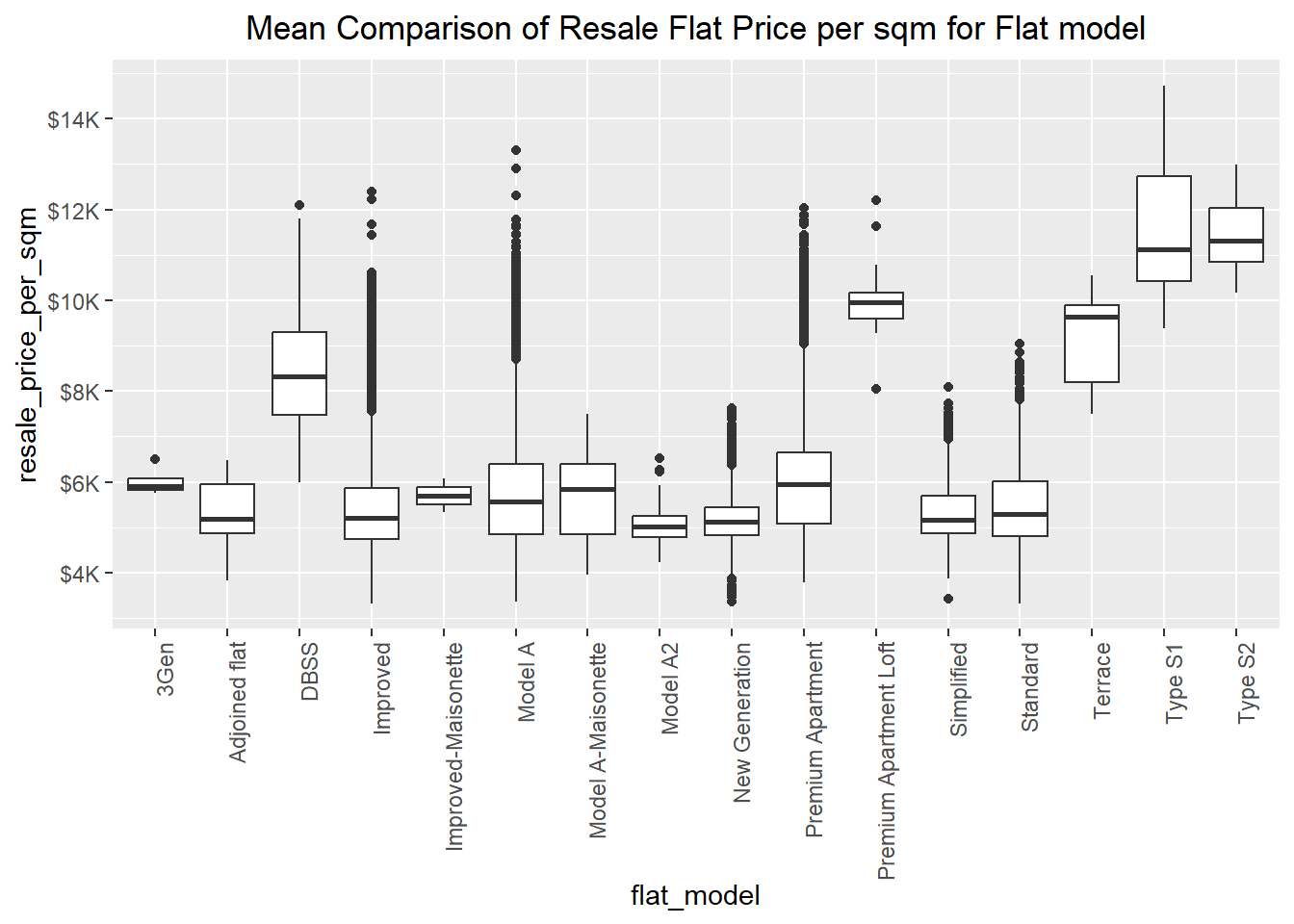
3.4.4 Mean resale flat price for different storey
In the code chunk below, boxplot of flat price for different storey range are displayed for comparison. For easier reading, the Y axis value are format in $K unit and X axis title are rotated 90 degree.
ggplot(new_flat_data, aes(x = storey_range, y = resale_price_per_sqm)) +
  geom_boxplot() +
  scale_y_continuous(
    labels = scales::label_dollar(scale = 1/1000, suffix = "K"),
    breaks = seq(2000, 20000, by = 2000)) +
  ggtitle("Mean Comparison of Resale Flat Price per sqm for Storey Range") +
  theme(axis.text.x = element_text(angle = 90, vjust = 1, hjust=1), plot.title = element_text(hjust = 0.5))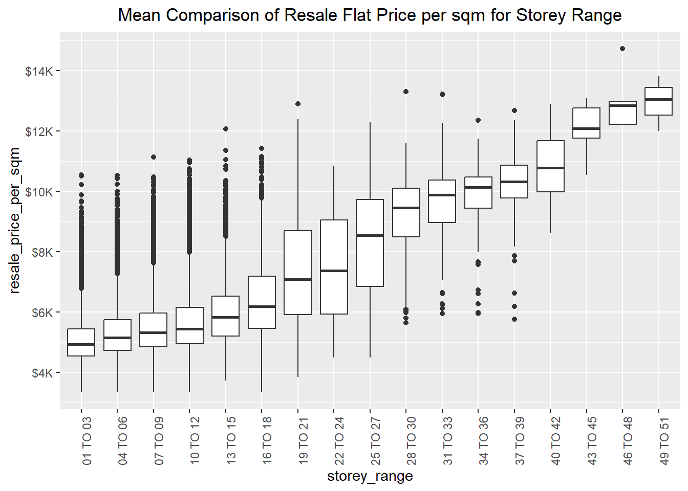
3.5 Scatterplot
3.5.1 Relationship between floor area and resale price per sqm
In the code chunk below, a scatterplot is built using ggplot2 with floor area and resale price per sqm on X & Y axis to visualize the relationship between two variables.
ggplot(data = new_flat_data,
       aes(x = floor_area_sqm, y = resale_price_per_sqm)) +
  geom_point() +
  geom_smooth(size = 1)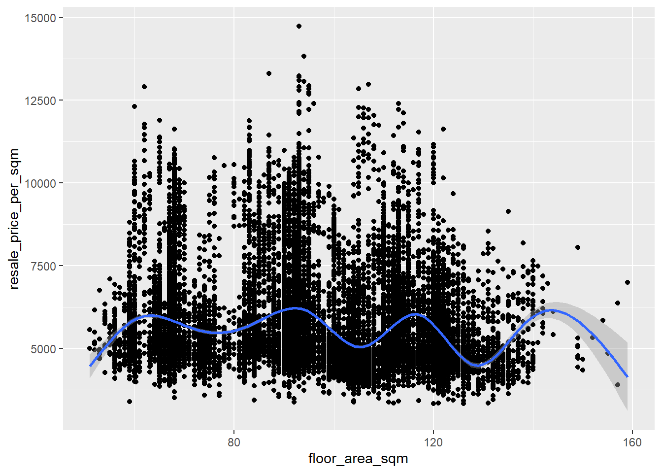
From the graph above, outliers from sqm = 150 and above has affected the correlation analysis. To generate more accurate result, I filter out data points for sqm = 150 and above
filter_new_flat_data <- new_flat_data %>%
  filter(floor_area_sqm < 150)
The scatterplot is rerun using the filtered data. Chart title is added for easier reading.
ggplot(data = filter_new_flat_data,
       aes(x = floor_area_sqm, y = resale_price_per_sqm)) +
  geom_point() +
  geom_smooth(size = 1) +
  ggtitle("Correlation between Floor Areq sqm and Resale Price per sqm")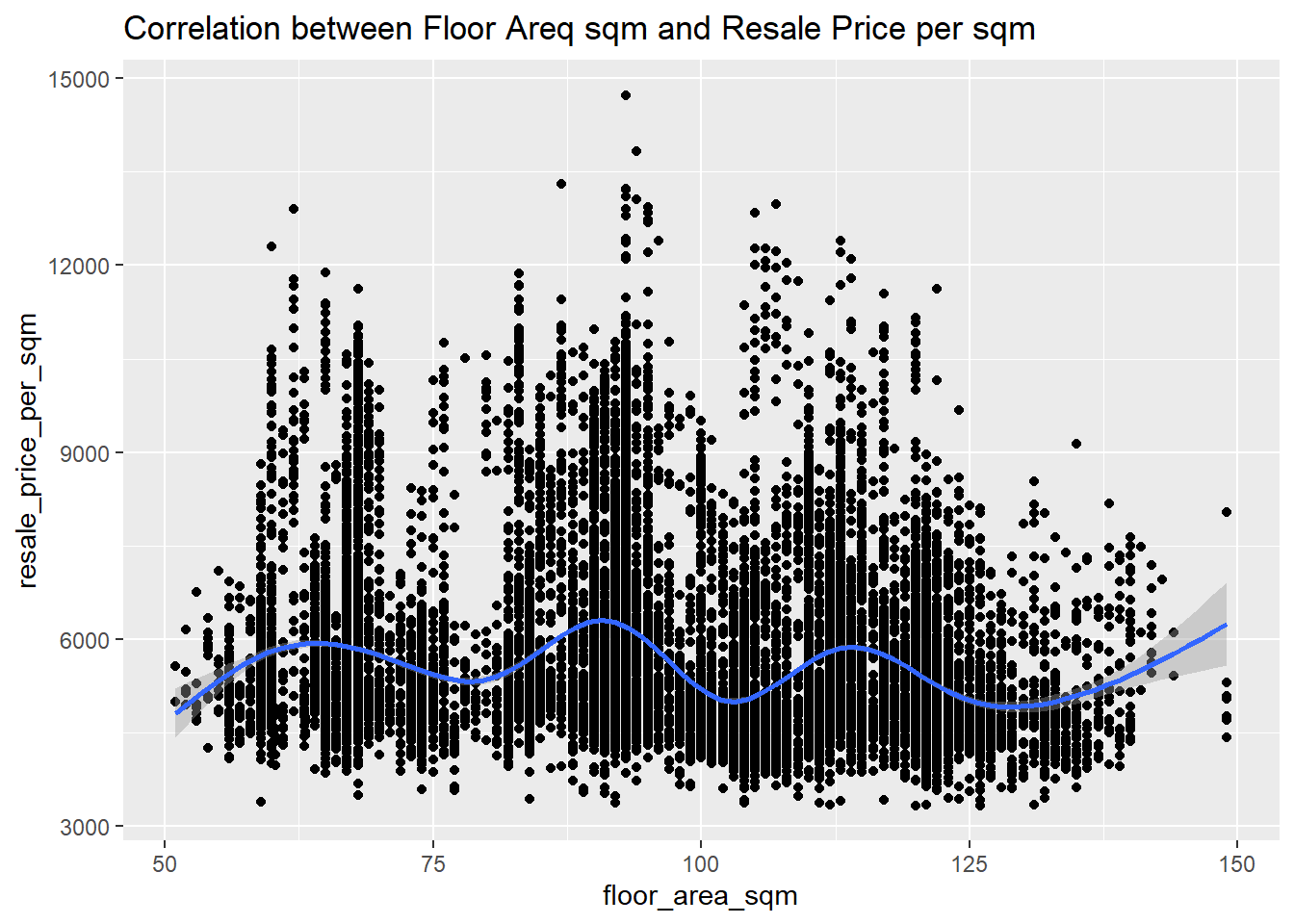
In the code chunk below, scatterplot is built using ggscatterstats() to visualize the significant test of correlation between floor area and resale price per sqm with the filtered data
ggscatterstats(
  data = filter_new_flat_data,
  x = floor_area_sqm,
  y = resale_price_per_sqm,
  marginal = FALSE
)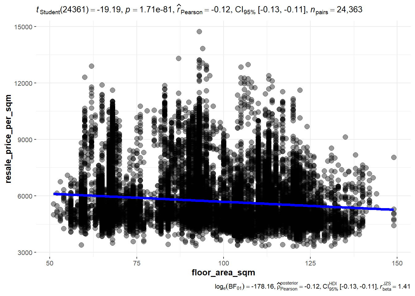
The above chart shows a p value < 0.05 and effect size = -0.12, which means there is a negligible negative correlation.
3.5.2 Relationship between remaining lease years and resale price per sqm
In the code chunk below, a scatterplot is built using ggplot2 with remaining lease years and resale price per sqm on X & Y axis to visualize the relationship between two variables.
ggplot(data = new_flat_data,
       aes(x = remaining_lease_years, y = resale_price_per_sqm)) +
  geom_point() +
  geom_smooth(size = 1)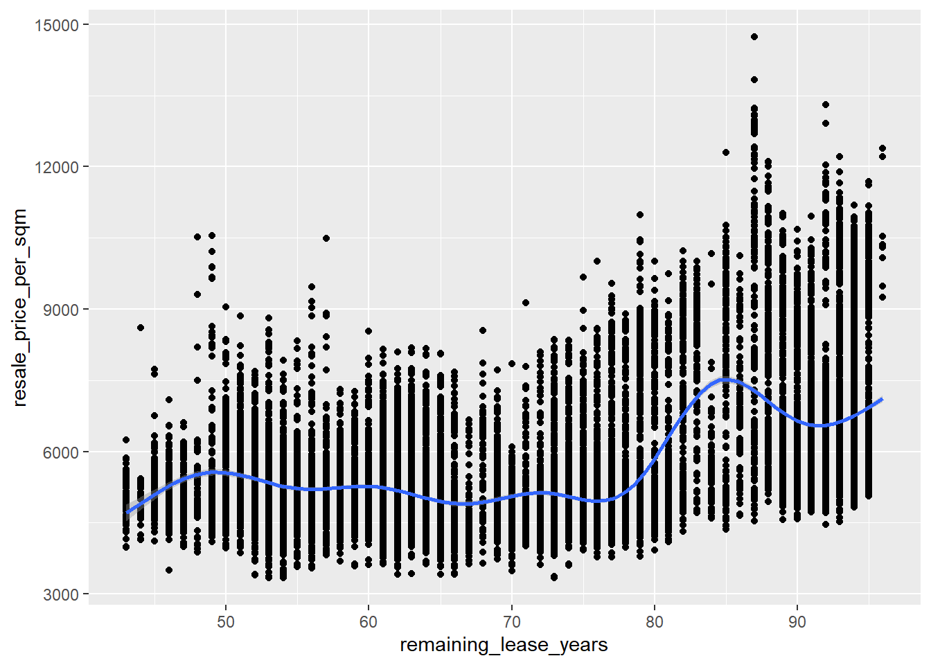
In the code chunk below, scatterplot is built using ggscatterstats() to visualize the significant test of correlation between remaining years and resale price per sqm.
ggscatterstats(
  data = new_flat_data,
  x = remaining_lease_years,
  y = resale_price_per_sqm,
  marginal = FALSE
)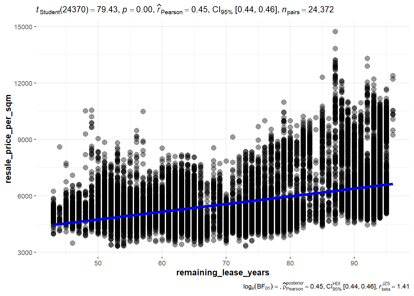
The above chart shows a p value < 0.05 and effect size = 0.34, which means there is a weak positive correlation.
4. Data Insights
1) Overall housing price distribution
In the first histogram, it shows a bell-shaped curve which is positively skewed.
The mean of resale price is around $5000.
All different flat type (3-room, 4-room and 5-room) shared similar pattern.
The statistical test suggests the housing price is not normally distributed.
2) Boxplot
The first boxplot suggests that average resale flat price is similar for different room type, which is statistically proven by the ANOVA test.
The second boxplot suggests that some area such as Central Area, Queenstown, Bukit Timah and Bukit Merah have a higher average resale flat price per sqm than other area.
The third boxplot suggests that some flat model such as Type S1 & Type S2, Premium Apartment Loft, Terrace and DBSS has a higher resale flat price per sqm.
The fourth boxplot suggests that higher storey range has a higher mean resale flat price per sqm.
These insights helps to explain what could be the possible driver that affects resale flat prices.
3) Scatterplot
The first scatterplot shows a negligible negative correlation between floor area and resale flat price per sqm
The second scatterplot shows a weak positive correlation between remaining lease years and resale price per sqm
These correlation could be too weak to prove whether there is a correlation between floor area and remaining lease years and resale flat prices.
5. Learning
In this exercise, I learn that we need to trial and error to find the best visualization for different type of data. For example, it won’t make sense if I use scatterplot for categorical data.
I also learn that we can leverage on visualization to improve the accuracy of statistical analysis. For example, we can identify outlier through scatterplot, and remove the outlier before we conduct statistical testing.
Moving on, I am interested to see what are visualization tools I can use to calibrate advanced analytics such as predictive models.